In my undergraduate coursework, I never took a course in error-correcting codes. It is possible that this is because I went to a small engineering school which doesn’t have a large course catalog. Thus, when my advisor asked me to look into the applicability of machine learning in LDPC polynomial generation, I needed to do some self-teaching. This post summarizes my learnings on LDPC and my thoughts on its connection to machine learning.

This post takes the following structure:

• Error correcting codes
• Low-Density Parity Check (LDPC) codes
• Design of LDPC and Machine Learning

1. Error correcting codes

In digital communications networks, much effort has gone into determining how to mitigate error. At the transmitter, digital messages are encoded as symbols, and in the case of an ideal channel, every transmitted symbol would arrive at the receiver unaltered, allowing for perfect reconstruction of the original message. In practice, the channel introduces noise, altering the transmitted symbol and introducing error in the message that is reconstructed at the receiver.

Figure 1: Hypothetical communications network including receiver, channel, and transmitter. Errors in the original message, \(m_x\), are induced by errors introduced during encoding at the transmitter, tranmission through the channel, or decoding at the receiver resulting in \(m_y\).

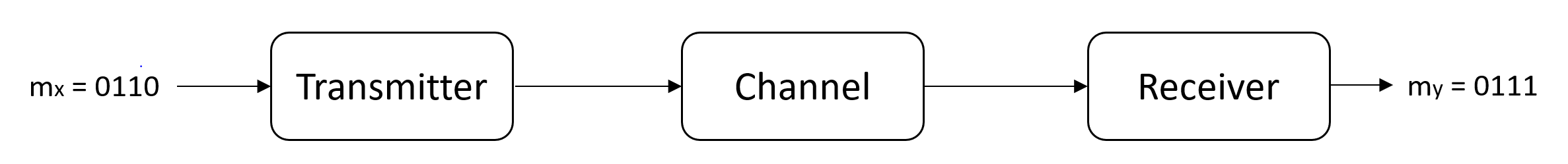
The possibility of such error motivates error-correcting codes (ECCs), which constitute a method of detecting and correcting errors in corrupted messages. The underlying premise is that a given transmitted message, \(m_x\), that is corrupted and interpreted as \(m_y\) might be augmented with redundant information (see Table 1).

$$\newcommand\T{\Rule{0pt}{1em}{.3em}} \begin{array}{|c|c|c|c|} \hline m_{x} & m_{x,aug} & m_y & m_{x,est} \T \\\hline 0 & 000 & 000 \T & 0 \\\hline 0 & 000 & 001 \T & 0 \\\hline 0 & 000 & 010 \T & 0 \\\hline 0 & 000 & 100 \T & 0 \\\hline 1 & 111 & 111 \T & 1 \\\hline 1 & 111 & 110 \T & 1 \\\hline 1 & 111 & 101 \T & 1 \\\hline 1 & 111 & 011 \T & 1 \\\hline \end{array} \\ $$ Table 1: A hypothetical ECC in which the original message, \(m_x\), is augmented to form a codeword \(m_{x,aug}\). A single bit of \(m_{x,aug}\) is corrupted, yielding \(m_{y}\) at the receiver. The estimated original message, \(m_{x,est}\), is taken as the codeword which is closest to the original \(m_{x}\).

The above ECC is defined by the column \(m_{x,aug}\). ‘\(000\)’ and ‘\(111\)’ are the valid codewords which comprise the code. These codewords vary from one another by three bits, which is the minimum Hamming distance of the code. In general, the Hamming distance is defined as the number of bits by which two codewords, \(m_1\) and \(m_2\), vary. This can also be viewed as the number of \(1\)’s resulting in an XOR operation between two codewords (i.e., \(m_1\oplus m_2\)).

The code can be assessed in terms of its error detection and error correction capabilities. Given minimum Hamming distance, \(d\):

• Error detection is the number of erroneous bits which the code can recognize (\(d-1\)).
• Error correction is the number of bits which the code can correct (\(\lfloor \frac{d-1}{2} \rfloor\)).

In the example code above (\(d=3\)), the error correction capability is \(d-1=2\), and the error correction capability is \(\lfloor \frac{d-1}{2} \rfloor=1\).

Our example ECC has a few shortcomings, namely:

1. Inefficiency: The transmission of larger messages might become prohibitively expensive to transmit. For each bit, we send two additional bits
2. Ineffective: The error detection/correction capability is limited given the size of the code, as we only have two codewords, \(000\) and \(111\).

Turns out that there are better ways to construct ECCs which overcome these limitations~ Such ECCs can be classified in one of two ways:

1. Convolutional codes
2. Linear block codes

For the remainder of this article, we focus our attention on a particular family of linear block codes: Low-Density Parity Check codes.

2. Low-Density Parity Check (LDPC) codes

Parity check codes detect and correct errors by checking whether the decoded codewords satisfy a system of linear equations. Given codewords of length \(n\) comprised of symbols \({x_1, x_2, \dots, x_n}\), the codewords satisfy the parity check equations:

$$x_a \oplus x_b \oplus \dots \oplus x_z = 0$$

These equations are summarized by a parity matrix, \(H\), which specifies which code symbols are XOR’ed in performing the parity check. Consider the matrix of the following form:

$$H=\begin{bmatrix} 1 & 1 & 1 & 0 & 1 & 0 & 0 \\ 0 & 1 & 1 & 1 & 0 & 1 & 0 \\ 1 & 1 & 0 & 1 & 0 & 0 & 1 \\ \end{bmatrix}$$

Any codeword \(m_x\) in the parity check code should yield a zero-vector when multiplied against \(H\) will yield a zero-vector of length \(n\). For \(H\) above, the codewords will satisfy the following system of equations:

$$\begin{align} 0&=x_1\oplus x_2 \oplus x_3 \oplus x_5 \\ 0&=x_2\oplus x_3 \oplus x_4 \oplus x_6 \\ 0&=x_1\oplus x_2 \oplus x_4 \oplus x_7 \end{align}$$

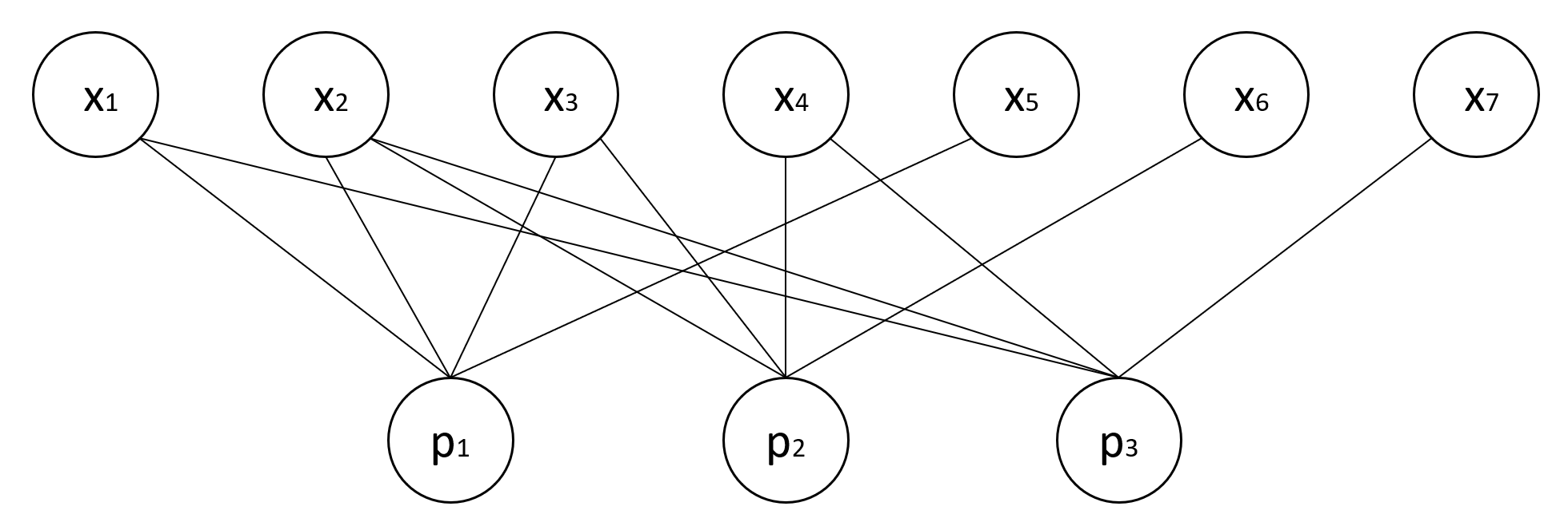
In other words, the valid codewords occupy the left null-space of \(H\). These codes can be defined by the tuple \((n,k,p)\) where \(n=\) number of variable nodes per codeword, \(k=\) number of data symbols per codeword, and \(p=\) number of parity check bits. The example code above is defined by the tuple \((7,4,3)\). Linear block codes may be visualized as Tanner graphs, which are bipartite graphs whose edges are defined by \(H\). For the \((7,4,3)\) code above, the corrseponding Tanner graph is given below:

Figure 2: Tanner graph for \((7,4,3)\) Hamming code. Variable and check nodes correspond to the columns and rows of \(H\), respectively. The 0-valued equations above are evaluated at the check nodes based on combinations of variable nodes \(x_i\).

So what makes LDPC codes ‘low density’? The density of \(H\) can be thought of as the proportion of \(1\)’s to \(0\)’s, meaning a low density code is primarily composed of \(0\)’s. Codes of low density have a lower likelihood of containing cycles, which have adverse effects when attempting to decode messages.

Decoding of LDPC codes is accomplished by belief propagation and variations thereof (e.g., the sum-product algorithm). Python implementations of this algorithm exist [3], and I hope to cover its utilization in a future post.

3. Design of LDPC and Machine Learning

So where does machine learning come into play? Without diving too deep into notation, the design of these LDPC codes involves the specifcation of degree polynomials which describe the sparsity of \(H\). The predominant algorithm used to optimize these polynomials is called density evolution [4]. Density evolution involves incrementally adjusting the coefficients in the degree polynomials and assessing how the Block Error Rate (BER) is affected.

This mechanism is reminiscent of reinforcement learning, a field of machine learning where an agent occupies a certain state and takes actions based on a policy in the hopes of maximizing its reward (or minimizing its penalty) [5]. In the case of LDPC design, one could treat the current state as the values of the polynomial coefficients, and the ‘agent’ could take action by adjusting the coefficients until an acceptably minimal BER is achieved.s

In the near future, I hope to have some preliminary results on a reinforcement learning approach to adjusting the degree polynomials.

4. References

• [1] J. K. Wolf, ‘An Introduction to Error Correcting Codes Part 3,’ UCSD ECE154C Lecture slides. Spring 2010. Link
• [2] B. P. Lathi, and Z. Ding, ‘Low-Density Parity Check (LDPC) Codes’, Ch 14, Sec 12 of Modern Digital and Analog Communications Systems.
• [3] ilyavka, sumproduct Repository on Github
• [4] T. J. Richardson, M. A. Shokrollahi and R. L. Urbanke, “Design of capacity-approaching irregular low-density parity-check codes,” in IEEE Transactions on Information Theory, vol. 47, no. 2, pp. 619-637, Feb 2001.
• [5] R. S. Sutton and A. G. Barto, “Reinforcement Learning: An Introduction,” MIT Press, Second Edition.