Approximating the Void: A Paper Review

28 Jun 2019

Intro Python Machine Learning GAN

1. Introduction

Ever since Goodfellow’s seminal paper [1], Generative Adversarial Networks (GANs) have been widely applied in the processing, synthesis, and classification of images, text, and audio. The premise of a GAN is to run a minmax game between two agents. One agent, the discriminator, tries to minimize a certain metric while the other agent, the generator, tries to maximize another metric. The generator is trained to discern whether or not a given sample is real or fake, and the generator learns to synthesize realistic samples which can fool the discriminator.

At the intersection of wireless communications and machine learning, researchers from DeepSig have demonstrated neural network architectures which can ‘learn’ a modulation scheme [2,3], but their work relied on analytic approximations of the channel model, limiting the trainability of the encoding/decoding networks since gradient could not be backpropagated through the channel.

To remedy this, the DeepSig team used a GAN to approximate the channel [4]. (As far as I am aware, IEEE does not give a “Most Likely to Become a Sci-fi Series” award to conference paper titles, but if they did, then ‘Approximating the Void’ would be a strong contender.) This post aims to recreate some of the results from DeepSig’s forray into GANs and to investigate whether or not their technique generalizes to different types of channel distributions.

2. Methods

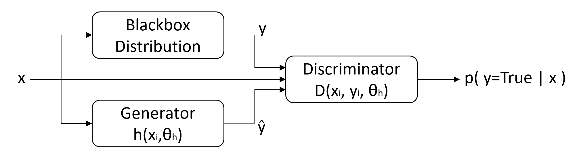
The architecture adopted in [4] is pictured in Figure 1. The “blackbox distribution” represents input-output ($x$ and $y$) samples from a real channel, and the generator is trained to produce estimates of the channel’s outputs ($\hat{y}$).

For this post, I utilitzed a BPSK modulation scheme, meaning $x \in [-1,1] $.

GAN Diagram for channel estimation.

Figure 1: Structure of GAN used to approximate blackbox distribution (i.e. channel distribution).

Optimization was done using the Adam optimizer with learning rate 1e-4, and during each epoch, we switch between the following two loss functions:

$\begin{align} \nabla_{\theta_D}\frac{1}{N}\sum_{i=0}^{N} \left[\log (D(x_i,y_i,\theta_D))\log (1-D(x_i,G(x_i,\theta_G),\theta_D))\right]\\ \nabla_{\theta_G}\frac{1}{N}\sum_{i=0}^{N} \log (1-D(x_i,G(x_i,\theta_G),\theta_D)) \end{align}$

where $\theta_G$ and $\theta_D$ represent the parameters for the generator and the discriminator, respectively. The network’s hyperparameters are listed in Tables 1 and 2. To get stochastic estimates ($\hat{y}$), the authors utilized a variational sampling layer comprised of Gaussian distributions. The inputs to this layer correspond to the mean and the variance of a Gaussian. I increased the dimensionality of the sampling layer and its preceding linear layer by a factor of two for reasons that I’ll touch on later.

Layer	Activation	Output Dimension
1	FC-ReLU	20
2	FC-ReLU	20
3	FC-ReLU	20
4	FC-Linear	64
5	Sampling	32
6	FC-ReLU	80
7	FC-Linear	1

Table 1: Generator hyperparameters.

Layer	Activation	Output Dimension
1	FC-ReLU	80
2	FC-ReLU	80
3	FC-ReLU	80
4	FC-Linear	1

Table 2: Discriminator hyperparameters.

I could not find a built-in activation function in Keras, so I used an snippet from a Keras example, variational_autoencoder_deconv.py.

def sampling(args):
    """Reparameterization trick by sampling fr an isotropic unit Gaussian.
    # Arguments
        args (tensor): mean and log of variance of Q(z|X)
    # Returns
        z (tensor): sampled latent vector
    """

    z_mean, z_log_var = args
    batch = K.shape(z_mean)[0]
    dim = K.int_shape(z_mean)[1]
    # by default, random_normal has mean=0 and std=1.0
    epsilon = K.random_normal(shape=(batch, dim))
    return z_mean + K.exp(0.5 * z_log_var) * epsilon

This activation function, or any custom activation function, can be associated with a given layer by using the Lambda layer. I did this in my build_generator method as follows:

    def build_generator(self):
        # new code: functional model
        g_dim=self.gen_dims
        inputs = Input(shape=(self.mod_dim,))
        x = Dense(g_dim['fc_relu1'], activation='relu')(inputs)
        x = Dense(g_dim['fc_relu1'], activation='relu')(x)
        x = Dense(g_dim['fc_relu1'], activation='relu')(x)
        x = Dense(g_dim['fc_lin1'], activation='linear')(x)
        # zero-mean, unit variance init weights for sampling layer
        z_mean = Dense(g_dim['fc_samp'], name='z_mean')(x)
        z_log_var = Dense(g_dim['fc_samp'], name='z_log_var')(x)
        # use reparameterization trick to push the sampling out as input
        z = Lambda(sampling, output_shape=(g_dim['fc_samp'],), name='z')([z_mean, z_log_var])
        x = Dense(g_dim['fc_relu2'], activation='relu')(z)
        predictions = Dense(g_dim['fc_lin2'], activation='linear')(x)
        model = Model(inputs=inputs,outputs=predictions)
        return model  

The learning rates (1e-4 to 5e-4) and optimizer (Adam) were kept consistent with the paper’s. I will make the full code available at a later date in the near future, but I largely based the architecture off wgan.py in the Keras-GAN repo.

3. Results

AWGN Channel

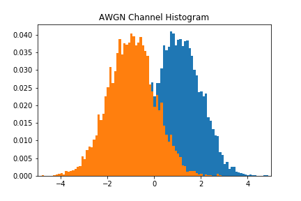
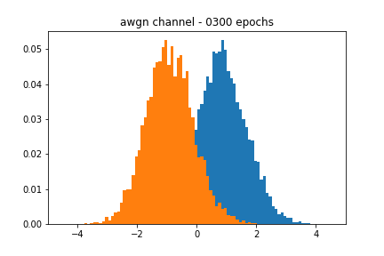
Since the generator’s variational layers of the GAN are Guassian, the network provides a good estimate of the AWGN channel. The blackbox distribution for the AWGN channel was built using samples from

$y=x+\mathcal{N}(0,1).$

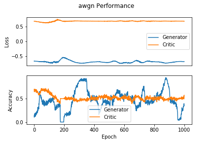
Figure 2 showcases the blackbox and the approximate distributions, both of which have a similar mean and variance. Figure 3 shows the performance of the network over time. We see that the accuracy of the discriminator hovers around 0.5, meaning that it cannot discriminate between a real or a fake sample.

Figure 2: Blackbox distribution and GAN-approximated distribution at 300 epochs for AWGN channel. Learning rate: 1e-4.

Loss and accuracy during GAN training for AWGN channel.

Evolution of GAN's AWGN approximate channel distribution for 1000 epochs.

Figure 3: Loss and accuracy during training and evolution of approximate distribution for AWGN channel (1000 epochs).

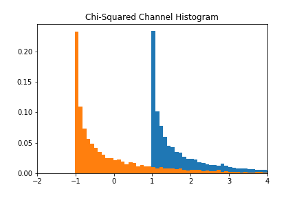
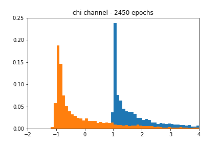
Chi-squared channel

The authors of [4] also showed their network’s capacity to perform on a non-Gaussian distribution: the chi-squared distribution,

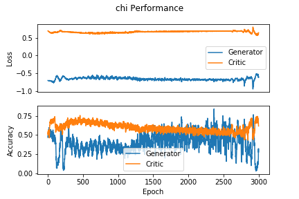
$\begin{align} y&=x(t)+\frac{1}{2^{k/2}\Gamma(k/2)}z^{k/2}e^{-z/2}\\ z&\thicksim \mathcal{N}(0,1). \end{align}$

We see from Figure 4 that the GAN-based approximation can find a decent representation of the chi-squared channel. Figure 5 shows that despite using the same learning rate as the AWGN case, the accuracy of the approximation is much noisier in the chi-squared case.

Blackbox distribution for chi-squared channel.

Trained approximation of chi-squared channel.

Figure 4: Blackbox distribution and GAN-approximated distribution at 2450 epochs for chi-squared channel. Learning rate: 1e-4.

Loss and accuracy during GAN training for chi-squared channel.

Evolution of GAN's approximate chi-squared channel distribution for 3000 epochs.

Figure 5: Loss and accuracy during training and evolution of approximate distribution for chi-squared channel (3000 epochs).

Fading channel

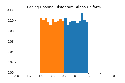
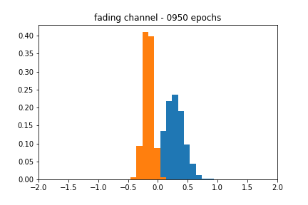
My original motivation for this post was to see what other types of distributions this architecture could model. I generated a ‘fading’ channel distribution, which was sampled as

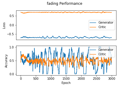
$\begin{align} y &= \alpha x(t) \\ \alpha & \thicksim \text{Uniform}(0,1). \end{align}$

The blackbox distribution for this can be seen in Figure 6. The approximation does a reasonable job of finding the actual mean, but the shape of the estimate is still characteristic of a Gaussian. Figure 7 corroborates this behavior, as the accuracy over epochs varies wildly, and the different distributions evolve within the range of their respective uniform distributions but never achieve the proper shape.

Blackbox distribution for fading channel.

Trained approximation of fading channel.

Figure 6: Blackbox distribution and GAN-approximated distribution at 950 epochs for fading channel. Learning rate: 1e-4.

Loss and accuracy during GAN training for fading channel.

Evolution of GAN's approximate fading channel distribution for 3000 epochs.

Figure 7: Loss and accuracy during training and evolution of approximate distribution for fading channel (3000 epochs).

4. Discussion/Future Work

Non-Gaussian distributions

So can we model non-Gaussian distributions with the given architecture? The chi-squared channel is fundamentally Gaussian-esque, as it involves sampling from a normal distribution and squaring those samples, so we take the results of the chi-squared test with a grain of salt.

The results of the fading channel tests make the generalizability of the architecture seem doubtful. The original motivation for increasing the dimensionality of the sampling layer was to see if more Guassians would give the generator enough degrees of freedom to replicate a uniform distribution, but doubling this value did not do the trick.

In future work, I might take a different tack at answering this question. Some thoughts:

Can we use different distributions in variational layer (e.g., uniform) to model non-Gaussian channels?
Does higher dimensionality of the sampling layer have an effect?

How do I stop this thing?

I cherry-picked the figures at particular epochs since they closely resembled their respective blackbox distributions. In a real-world scenario, we would like the network to stop training when its accuracy passes a certain threshold, but my results implementing such an approach were spotty. It is possible that I was not using the right accuracy metric in Keras, which I believe defaults to binary_crossentropy.

5. References

[1]. I. Goodfellow, J. Pouget-Abadie, M. Mirza, B. Xu, D. Warde-Farley, S. Ozair, A. Courville, and Y. Bengio, “Generative adversarial nets,” in Advances in neural information processing systems, 2014, pp. 2672–2680.
[2]. T. J. O’Shea, K. Karra and T. C. Clancy, “Learning to communicate: Channel auto-encoders, domain specific regularizers, and attention,” 2016 IEEE International Symposium on Signal Processing and Information Technology (ISSPIT), Limassol, 2016, pp. 223-228.
[3]. S. Dörner, S. Cammerer, J. Hoydis and S. t. Brink, “Deep Learning Based Communication Over the Air,” in IEEE Journal of Selected Topics in Signal Processing, vol. 12, no. 1, pp. 132-143, Feb. 2018.
[4]. T. J. O’Shea, T. Roy and N. West, “Approximating the Void: Learning Stochastic Channel Models from Observation with Variational Generative Adversarial Networks,” 2019 International Conference on Computing, Networking and Communications (ICNC), Honolulu, HI, USA, 2019, pp. 681-686.