I have been working on deep learning in the context of CSI estimation in MIMO systems using FDD modulation schemes. While correlations between uplink and downlink are weaker than those in TDD schemes, spatial and spectral correlations still provide useful information. In [1], the authors train a network, DualNet, to leverage uplink and downlink reciprocity in estimating downlink CSI.

While trying to extend train DualNet on a 128 antenna dataset (the original implementation uses 32 antennas), I noticed that the training time became prohbitively long. For \(10^5\) samples, the estimated training time was 76 days. To speed up the training time, I wondered where I might be able to reduce the number of parameters in the network.

To cut down on trainable parameters, I needed to understand what sorts of activations the network was learning. If certain layers are largely inactive, then perhaps those layers can be removed. To visualize hidden layers, I retooled a tutorial [2] where the author visualizes the activations for a shape-classifying Convolutional Neural Network (CNN).

The DualNet Model

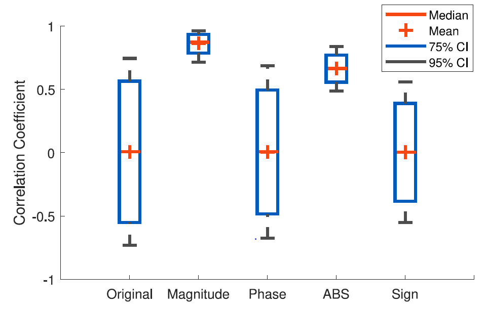
First, I provide a brief summary of DualNet. The premise of DualNet is that despite weak phase correlation between uplink and downlink, the magnitude correlation and absolute value correlations are high (see Figure 1).

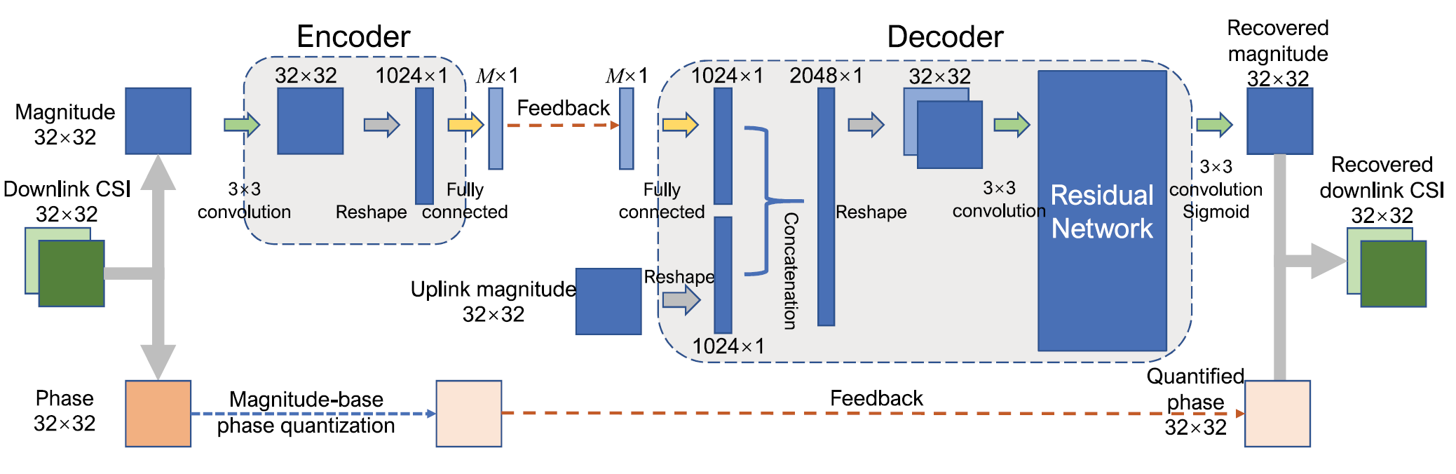
With this observation, DualNet is tailored to accept either the magnitude or the absolute value of CSI. The magnitude variant, DualNet-MAG, is shown in Figure 2. DualNet assumes that a user equipment (UE) will leverage a CNN (the Encoder) to compress the downlink feedback and that the base station (BS) will use another CNN (the Decoder) to use encoded downlink and raw uplink values to estimate the downlink.

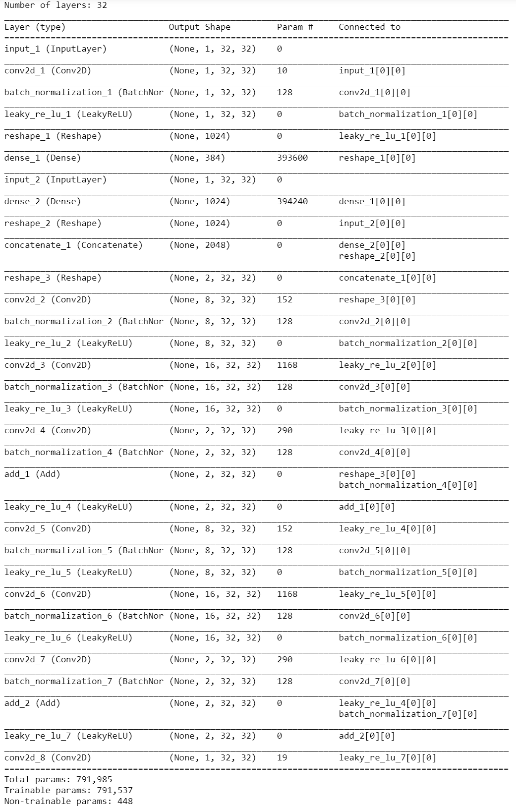
The Keras implementaion of DualNet-MAG and DualNet-ABS can be found in [3]. Assuming a compression ratio of \(1/4\), the network summary is shown in Figure 3. Even though there are only 32 antennas, the number of trainable parameters is already fairly large (\(\approx 8\cdot 10^5\)). However, the preponderance (\(\approx 99\%\)) of the parameters appear to be in the Dense layers.

The Activation Model

Now we look at layer-wise activations. After training the DualNet model, I pulled some samples from the validation set for the visualization. The code for this can be found in my fork of [3]. Below, I share some layer activations for a few layers of interest

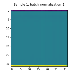
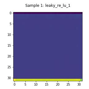
Input Residual Network (Encoder)

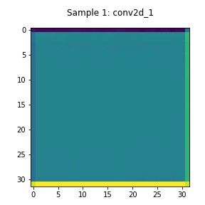
The encoder’s activations are shown in Figure 4. The layers’ outputs largely assume the same value except for the last row of the matrix. This means that the layer may not be contributing substantial information to the encoding.

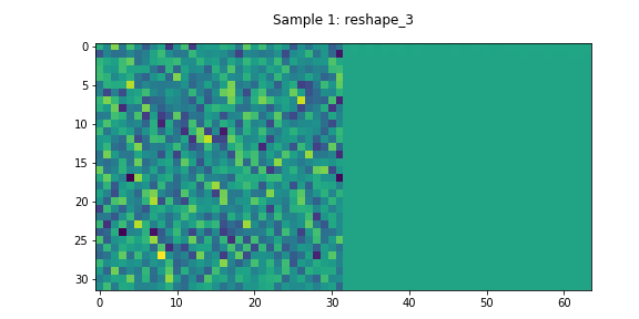
Dense Layer Output (Encoder)

The activations after the second dense network and the corresponding uplink CSI magnitude are shown in Figure 5. Despite the encoded downlink CSI having no apparent structure, the decoder is still able to reconstruct the accurate estimates of the downlink.

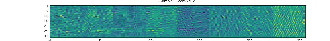
Residual Network (Decoder)

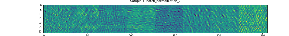
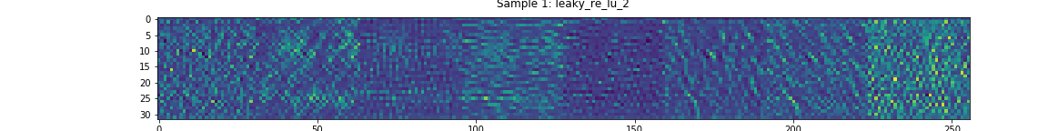
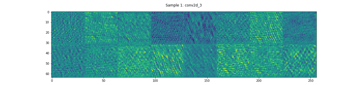
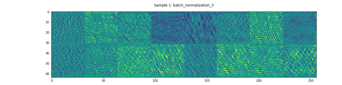
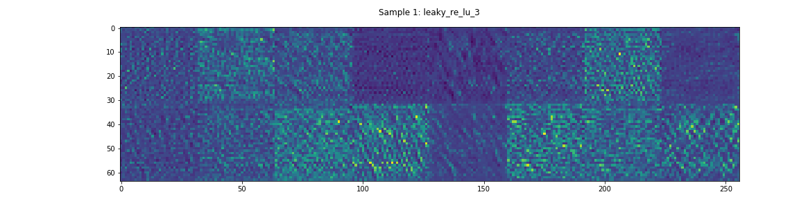
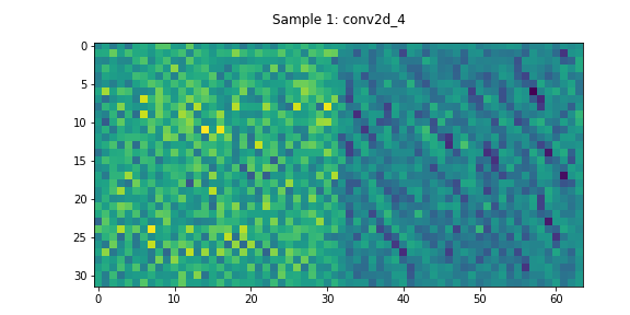
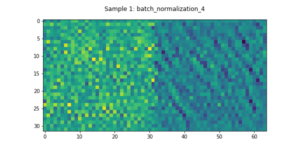
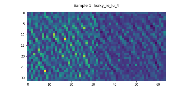
In this model, DualNet’s decoder has two daisy-chained residual networks. The activations through one of these networks can be seen in Figure 6. In contrast to the Encoder’s residual network, most of these layers appear to have non-negligible learned features.

Output Layer

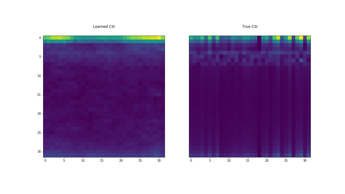
Finally, we compare the network’s output, the learned CSI, to the true downlink CSI in Figure 7.

Discussion

Dense layers: Based on the above visualization, the dense layers between the encoder and the decoder appear to contribute substantially to the encoding. It remains an open question what the minimum necessary dimension of this layer needs to be, so further work into changing the structure of the dense layers would be worthwhile given their large dimensionality.

Encoder layers: Anoter potential area of improvement could be the encoder. Based on Figure 4, it seems that the initial residual network is not contributing much information as its relu layer’s activations are sparse. Removing the convolutional layers from the encoder would reduce the complexity of the network and may improve training time. Given that the encoder is meant to operate at the UE, which is likely to have fewer computational resources than the BS, such an approach might be appealing.

References

• [1]. Z. Liu, L. Zhang and Z. Ding, “Exploiting Bi-Directional Channel Reciprocity in Deep Learning for Low Rate Massive MIMO CSI Feedback,” in IEEE Wireless Communications Letters, vol. 8, no. 3, pp. 889-892, June 2019.
• [2]. Pierobon, G. “Visualizing intermediate activation in Convolutional Neural Networks with Keras,” Medium. November 2018. Link
• [3]. DLinWL, Bi-Directional-Channel-Reciprocity